Ch02 預備知識 — Math

# Linear Algebra

Essential in deep learning and AI.

• Scalars (純量)
  • 標記：小寫 (x)
  • 基本運算如下:

    	# Creating two PyTorch tensors 'x' and 'y'
    	x = torch.tensor(3.0)
    	y = torch.tensor(2.0)
    	# Performing basic arithmetic operations using PyTorch tensors.
    	# 'x + y' adds the two tensors.
    	# 'x * y' multiplies the two tensors.
    	# 'x / y' divides tensor 'x' by tensor 'y'.
    	# 'x**y' raises tensor 'x' to the power of tensor 'y'.
    	x + y, x * y, x / y, x**y

• Vector
  • 標記：小寫粗體 ($\mathbf{x}$)
  • Each element often represents a dataset feature.
  • 基本運算如下:

    	x = torch.arange(3)
    	print(x)
    	# 'len(x)' returns the size of the first dimension of 'x', which is 3 in this case.
    	print(len(x))
    	# 'x.shape' returns the dimensions of 'x', which is (3,) indicating it's a 1-dimensional tensor with 3 elements.
    	print(x.shape)

• Matrices
  • 標記：大寫粗體 ($\mathbf{A}$)
  • 基本運算如下:

    	A = torch.arange(6).reshape(3, 2)
    	A, A.T # transpose (轉置)

• Tensors (張量)
  • Definition: 推廣到更高維度的 n 維 arrays.
  • 標記：特殊字體的大寫字母 (e.g., $\mathbf{X}$).
  • Applications: Images (3rd-order: 長寬和顏色), videos (4th-order), data batches.

  torch.arange(24).reshape(2, 3, 4)

• Reduction (降維)
  • Summation: Over vector, matrix, specific axes.
  • Mean: Calculating average, along specific axes.

  	x = torch.arange(3, dtype=torch.float32)
  	A = torch.arange(6, dtype=torch.float32).reshape(2, 3)
  	x.sum(), A.mean()

• Non-Reduction Sum
  • sum with keepdims=True ，用來保持張量的維度。
  • Broadcasting: Allows for operations on tensors of different shapes.
  • Cumulative Sum ( cumsum ): Calculates cumulative sum along a specified axis.

  	A = torch.arange(6).reshape(3, 2)
  	# Calculating the sum of elements in 'A' along axis 0 (column-wise sum) and keeping the same number of dimensions.
  	# 'A.sum(axis=0, keepdims=True)' sums up elements column-wise and 'keepdims=True' retains the 2D shape of the result.
  	# This will result in a 1x2 tensor.
  	sum_result = A.sum(axis=0, keepdims=True)
  	# Calculating the cumulative sum of elements in 'A' along axis 0 (column-wise).
  	# 'A.cumsum(axis=0)' computes the cumulative sum column-wise.
  	# This will result in a 3x2 tensor where each element in a column is the sum of all previous elements in that column.
  	cumsum_result = A.cumsum(axis=0)
  	sum_result, cumsum_result

• Dot Product
  • Def.: $\mathbf{x}^{\top} \mathbf{y} = \sum_{i=1}^d x_i y_i$
  • Applications: Weighted sum, cosine similarity (看相似度，因為 $\vec{x}\cdot \vec{y}=\|\vec{x}\|\|\vec{y}\|\cos{\theta}$, 最小值在 0^o; 最大值在 180^o → 值越接近 1 越相似，CNN 會用), projections, matrix multiplication.

  	x = torch.tensor([1,2,3])
  	y = torch.tensor([4,5,6])
  	torch.dot(x, y), torch.sum(x * y)

• Matrix-Vector Products
  • torch.mv(A, x) , A @ x

$$\mathbf{A}\mathbf{x} = \left[ \begin{array}{c} \mathbf{a}_1^{\top}\mathbf{x} \\ \mathbf{a}_2^{\top}\mathbf{x} \\ \vdots \\ \mathbf{a}_m^{\top}\mathbf{x} \\ \end{array} \right]$$

• Matrix-Matrix Multiplication

  $$C_{ij} = \sum_{k=1}^{n} A_{ik} \times B_{kj}$$

  	A = torch.arange(6, dtype=torch.float32).reshape(3, 2)
  	B = torch.ones((2,3))
  	print(A.dtype, B.dtype)
  	print(torch.mm(A,B), A@B, sep="\n")

  • @表 tensor 乘以 tensor，所以 vector 和 matrix 皆可使用。
• Norms (範數，即距離)
  • Def.: Function that assigns a non-negative length to a vector.
  • Vector Norms
    • Euclidean (歐氏距離，L2 norm)

    $$\ell_2=\sqrt{x^2+y^2}$$

    • Manhattan (曼哈頓，L1 norm)

    $$\ell_1=|x|+|y|$$

    • 推廣到 $\ell_p$ norm

    $$\ell_p=\|\mathbf{x}\|_p = (\sum_{i=1}^n |x_i|^p)^{1/p}$$

  • Matrix Norms: Frobenius norm

    $$\|\mathbf{X}\|_{\mathrm{F}} = \sqrt{\sum_{i=1}^m \sum_{j=1}^n x_{ij}^2}$$

  • Applications: Objective functions (目標函數), regularization (正規化), feature scaling (特徵縮放), distance metrics (距離函數), loss function.

  	x = torch.arange(3) #arange 預設是 int, 但 norm 要 float 才能算
  	print(x.dtype)
  	# print(torch.norm(x), torch.abs(x).sum()) # ERROR!
  	print( torch.norm(x.to(torch.float32)) ) # Euclidean, 5**(1/2)
  	print( torch.abs(x.to(torch.float32)).sum() ) # element-wise abs

# Calculus

Derivatives (導數) and partial derivatives (偏導數), plays a vital role in deep learning and AI.

• Derivatives
  • Def.: rate of change of f(x) with respect to x.
  • Slope of the tangent to the curve of f(x) at x.
  • 定義公式:

  $$f'(x) = \lim_{h \to 0} \frac{f(x+h) - f(x)}{h}$$

  	import numpy as np
  	def f(x):
  	return 3*x*x - 4*x
  	# Loop through values of h, starting from 10^-1 to 10^-6, decrementing by powers of 10
  	# This loop is used to calculate the numerical approximation of the derivative of the function f at x = 1,
  	# by applying the difference quotient formula: (f(x+h) - f(x)) / h
  	for h in 10.0**np.arange(-1, -6, -1):
  	numerical_limit = (f(1+h) - f(1)) / h
  	# Print the value of h and the calculated numerical limit
  	# The output shows how the approximation of the derivative at x = 1 becomes more accurate as h gets smaller.
  	print(f'h={h:.5f}, numerical limit={numerical_limit:.5f}')

• 常見導數和微分規則
  • Constant Rule: $\frac{d}{dx}C = 0$ for constant $C$.
  • Power Rule: $\frac{d}{dx}x^n = nx^{n-1}$ for $n \neq 0$.
  • Exponential and Logarithmic Functions: $\frac{d}{dx}e^x = e^x$, $\frac{d}{dx}\ln x = x^{-1}$.
  • Constant Multiple Rule: $\frac{d}{dx}[Cf(x)] = C\frac{d}{dx}f(x)$.
  • Sum Rule: $\frac{d}{dx}[f(x) + g(x)] = \frac{d}{dx}f(x) + \frac{d}{dx}g(x)$.
  • Product Rule: $\frac{d}{dx}[f(x)g(x)] = \frac{d}{dx}f(x)g(x) + f(x)\frac{d}{dx}g(x)$.
  • Quotient Rule: $\frac{d}{dx}\frac{f(x)}{g(x)} = \frac{\frac{d}{dx}f(x)g(x) - f(x)\frac{d}{dx}g(x)}{g^2(x)}$.
• 在深度學習上的應用
  1. Gradient Descent: 計算損失函數相對於權重的導數。
  2. Backpropagation: 使用 chain rule 進行高效梯度計算。
  3. Model Behavior: 透過導數理解輸入輸出關係。
  4. Optimization: 使用導數求函數最小值 / 最大值。
• Partial Derivatives (偏微分)
  • Def.: Derivative of a multivariable function $f(x_1, x_2, ..., x_n)$ with respect to one variable, treating others as constant.

  $$\frac{\partial y}{\partial x_i} = \lim_{h \rightarrow 0} \frac{f(x_1, \ldots, x_{i-1}, x_i+h, x_{i+1}, \ldots, x_n) - f(x_1, \ldots, x_i, \ldots, x_n)}{h}$$

  • 符號: $\frac{\partial y}{\partial x_i}, \partial_{x_i} f, f_{x_i}$, etc.
• Gradients (梯度)
  • Def.: Vector of partial derivatives for a function $f: \mathbb{R}^n \rightarrow \mathbb{R}$.
  • Notation ($\nabla$ 念 nabla or del )

  $$\nabla_{\mathbf{x}} f(\mathbf{x}) = [\partial_{x_1} f(\mathbf{x}), ..., \partial_{x_n} f(\mathbf{x})]^\top$$

  • 多變數函數的微分規則
    Matrix Derivatives:
    • $\mathbf{A} \in \mathbb{R}^{m \times n}$，$\nabla_{\mathbf{x}} \mathbf{A}\mathbf{x} = \mathbf{A}^\top$.
    • $\mathbf{A} \in \mathbb{R}^{m \times n}$，$\nabla_{\mathbf{x}} \mathbf{x}^{\top} \mathbf{A} = \mathbf{A}$.
    • $\mathbf{A} \in \mathbb{R}^{n \times n}$，$\nabla_{\mathbf{x}} \mathbf{x}^{\top} \mathbf{A}\mathbf{x} = (\mathbf{A} + \mathbf{A}^\top)\mathbf{x}$.
    • $\nabla_{\mathbf{x}}\|\mathbf{x}\|^2 = \nabla_{\mathbf{x}} \mathbf{x}^{\top}\mathbf{x} = 2\mathbf{x}$.
  • Frobenius Norm: $\nabla \mathbf{X}\|\mathbf{X}\|_{\mathrm{F}}^2 = 2\mathbf{X}$.
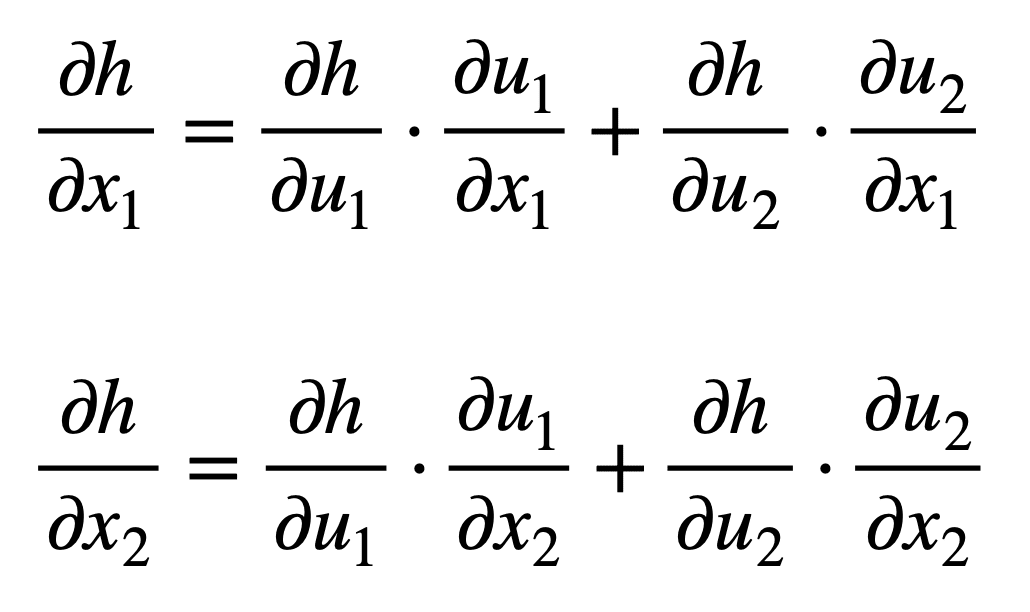
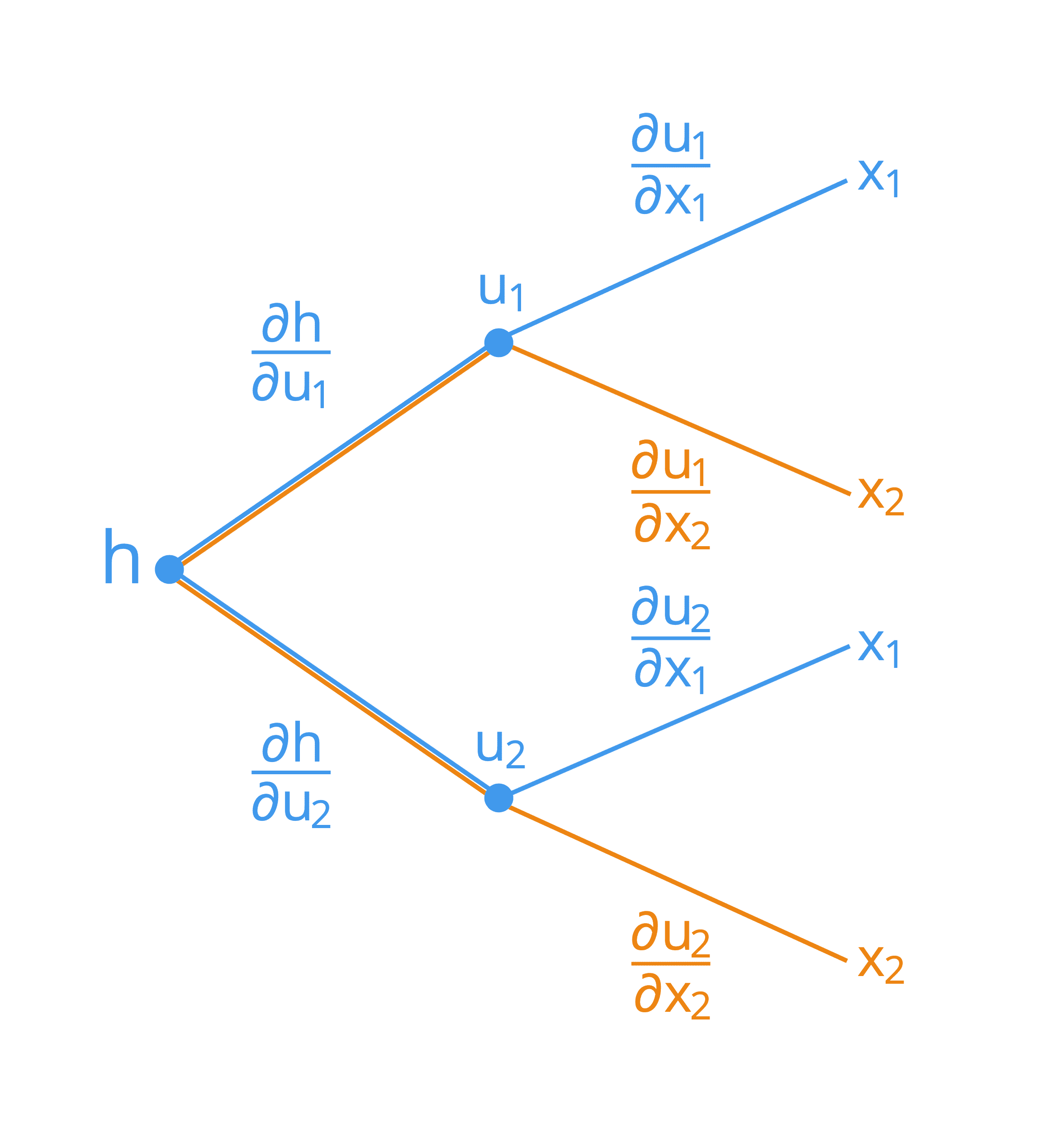
• Chain Rule
  • Application in Deep Learning
    • Backpropagation: Gradient computation in neural network training.
    • Gradient Descent: Weight update using computed gradients.
    • Model Sensitivity: Insights into model's sensitivity to inputs.
  • Single Variable: For $y = f(g(x))$, $\frac{dy}{dx} = \frac{dy}{du} \frac{du}{dx}$，where $u=g(x)$.
  • Multivariate Functions

  $$\frac{\partial y}{\partial x_i} = \sum_{j=1}^m \frac{\partial y}{\partial u_j} \frac{\partial u_j}{\partial x_i}$$

  • Vector Form: $\nabla_{\mathbf{x}} y = \mathbf{A}^T \nabla_{\mathbf{u}} y$, where $\mathbf{A}$ contains the derivatives of $\mathbf{u}$ with respect to $\mathbf{x}$.

$$A = \begin{bmatrix} \frac{\partial u_1}{\partial x_1} & \frac{\partial u_1}{\partial x_2} & \cdots & \frac{\partial u_1}{\partial x_n} \\ \frac{\partial u_2}{\partial x_1} & \frac{\partial u_2}{\partial x_2} & \cdots & \frac{\partial u_2}{\partial x_n} \\ \vdots & \vdots & \ddots & \vdots \\ \frac{\partial u_m}{\partial x_1} & \frac{\partial u_m}{\partial x_2} & \cdots & \frac{\partial u_m}{\partial x_n} \\ \end{bmatrix}$$

$$\nabla_{\mathbf{u}} y = \begin{bmatrix} \frac{\partial y}{\partial u_1} \\ \frac{\partial y}{\partial u_2} \\ \vdots \\ \frac{\partial y}{\partial u_m} \\ \end{bmatrix}$$

• Chain rule 圖示

# Auto Differentiation (自動微分)

# Bonus 2 題目

Give the function $f(x)=\cos(2x^{2}−x+3)+\sqrt{\exp(\sin(3x))}$
Please implement the gradient descent method to find the local minimum of this function give the initial $x_0=1$ and $x_0=−1$.

Hint:

(1) You must use the definition $\frac{df}{dx}=\frac{f(x+h)-f(x)}{h}$ to calculate the derivative of $f(x)$.
(2) A draft of the gradient descent method (please modify it on your own):

stop = False

x = x0 # initial value of x

alpha = 0.1 # set the learning rate to a small constant

t = 1

while not stop:

  f = f(x)

  df = the derivative of f(x) at x

  print("Iteration", t, ": f(x) = ", f, "df = ", df) # print the current function value and gradient

  if |df|<= 1e-5: # check if the gradient is almost zero (i.e., local minimum)

    stop = True

  else:

    x = x - alpha*df

    t = t + 1

print("the local minimum ", f, "is found at x = ", x)

解答地址: Colab

ref
矩陣微分 1 https://www.youtube.com/watch?v=t8fQliDkvoE
2 https://www.youtube.com/watch?v=2Wbx4waHhcY